Opening, Displaying and Saving Molecules and Views
Customizing and Manipulating Molecule Views
GaussView contains a variety of controls and features for customizing the displays in view windows. These may be accessed via the View menu, and also via toolbar icons in some cases. The View menu may also be accessed by clicking the right mouse button in an open area of any view window or other molecule display.
Centering the Molecule
The Center button and the View=>Center menu item centers and resizes the image in the active view window to make the most efficient use of the workspace.
Viewing Optional Display Items
Several View menu options toggle the display of optional items within a view window:
- View=>Hydrogens: Display of hydrogen atoms in the view window (initially on).
- View=>Dummies: Display of dummy atoms if present (initially on).
- View=>Labels: Display numeric labels indicating atom sequence numbers (initially off).
- View=>Symbols: Display the chemical symbol for each atom (initially off).
- View=>Bonds: Display bonds between atoms (initially on).
- View=>Cartesian Axes: Display X,Y,Z axes (initially off). This feature is illustrated in Figure 43. Initially, the origin of the axes is in an arbitrary position (sometimes located on atom 1), and it remains fixed despite changes to the molecule. Use the Edit=>Reorient menu item to move the origin to the molecule’s current center of mass.
- View=>Stereochemistry: Display the chirality of any chiral centers (initially off).
- View=>Positioning Tools: Open positioning toolbar in view window (initially off).
You can specify default values for these items via the General panel of the Display Format dialog (View menu) or the Display Format pane of the Preferences. You can also exclude labels and symbols on hydrogen atoms or hydrogen and carbon atoms using the Exclude View Labels and Exclude View Symbols items in the Text panel of the Display Format preferences (both default to excluding no atom types). Finally, the size of textual labels can be adjusted using the Size field in the Text panel of the Display Format preferences.
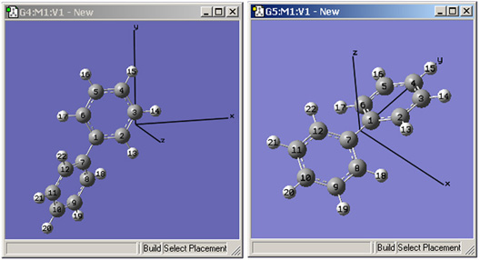
Figure 43. Displaying Cartesian Axes
These windows illustrate GaussView’s Cartesian Axes display option. The window on the left shows the initial position of the axes (which is quite arbitrary), and the one on the right shows the origin’s new position after using the Edit=>Reorient menu item.
Molecule Positioning Tools
Figure 44 illustrates the molecule positioning toolbar, which is accessed with the View=>Positioning Tools menu item.

Figure 44. The Positioning Toolbar
For all of the tools, the view’s X, Y and Z directions are the horizontal, vertical and depth of the window, and the molecule X, Y and Z directions are those indicated by the Cartesian axes. The various controls are described individually below (moving across the toolbar from left to right):
- The Quick popup contains items which center the molecule in one or more view directions or align axes on the molecule with that of the view. For example, the Center and Center X items center the molecule within the window and with respect to the window’s X-axis (i.e., horizontally), while the Mol X -> View Z item aligns the molecule's X-axis with the view window’s Z-axis. Other items work analogously.
- The second popup menu indicates whether the molecule will be rotated or translated in order to perform the repositioning when the Apply button is pushed. The next two fields also control the operation.
- The Around field specifies the axis about which the molecule will be rotated (active when the previous popup is set to Rotate). When Translate is selected in the initial field, then the label changes to Along.
- The By field specifies the amount of rotation or translation.
- The final slider provides another way to specify the amount of movement. As you adjust the slider, the molecule moves immediately in the direction and manner specified by the first two fields (and the By field is ignored).
Molecule Display Formats
The Display Format button and the View=>Display Format menu item both open the Display Format dialog. Each panel in this dialog also has a twin within the Display preferences. We will consider the General, Text and Molecule panels here and will consider the Surface panel later in this book.
The General Panel
The items in the General panel control molecule display quality, additional items displayed in addition to the atoms (as mentioned above) and the fog feature. It is illustrated in Figure 45.
The options in top part of this panel govern how the molecule appears both when it is being moved in the view window by mouse action and when it is not moving. On slower systems, it can be often useful to set the slider more toward the Realistic end of the scale for Stationary Object Display and more toward the Fast end of the scale for Moving Object Display.
The Smooth checkboxes enable/disable smoothing in the display, and the Spotlight checkboxes enable/disable simulated spotlighting on the window contents.
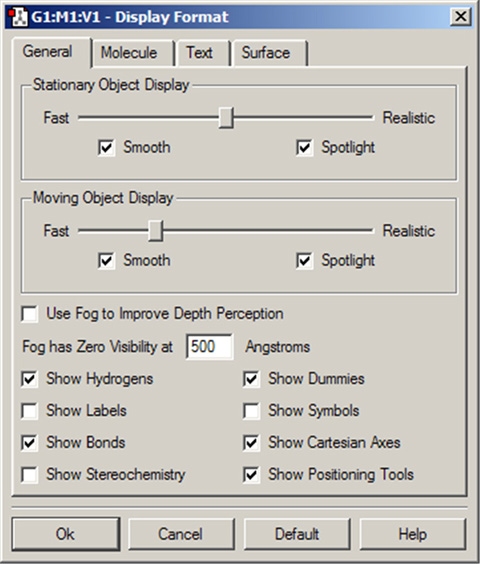
Figure 45. Display Format General Panel
The Use Fog to Improve Depth Perception checkbox causes more distant atoms in the view window to recede to invisible, allowing nearer atoms to become more distinct. The Fog has Zero Visibility at field controls the depth at which atoms become completely invisible.
This feature is illustrated in Figure 46. In this example, the lefthand illustration shows the molecule with the fog feature disabled. In the righthand illustration, fog is turned on, and the frontmost atoms are much more distinct than more distant ones.
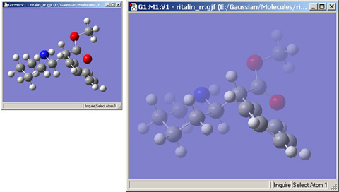
Figure 46. The Fog Depth Display Feature
Compare the display types between the two windows to understand the effect of fog.
The Molecule Panel
The options in this panel control how atoms and bonds appear in the view window. The three popup menus specify how atoms in each of the three ONIOM layers will be displayed. If the ONIOM facility is not being used, then the setting for the High Layer is used. The Molecule panel is shown in Figure 47.
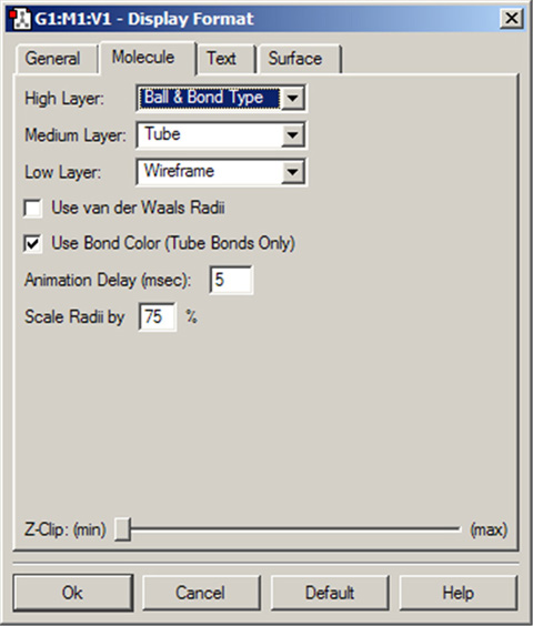
Figure 47. The Display Format Molecule Panel
The various items in this panel control various aspects of molecule displays.
The layer display settings are also used by some other GaussView features unrelated to ONIOM (e.g., displaying atoms at the boundaries of PBC unit cells).
The various supported display types are:
- Ball & Stick: Molecule appears as a ball and stick model, with all types of bonds represented by
single sticks. This is the default.
- Ball & Bond Type: Molecule appears as a ball and stick model with single bonds represented by single sticks, and multiple bonds represented by multiple sticks, or in the case of aromatic systems, by dotted lines.
- Tube: Molecule appears as a tube model with no indication as to bond type. Atom types are indicated by color bands on the tubes.
- Wireframe: Molecule appears as a series of thin lines, colored by atom type and indicating bond type via the number of lines.
- None: Atoms are invisible (useful only with multilayer models).
The Use Vanderwaals Radii checkbox and Scale Radii by field cause the atoms in the view window to be displayed at the indicated scaling of the van der Waals covalent radii. Using a scaling value of 150%-200% will produce a space filling-like molecular display, as in Figure 48.
Figure 48. A CPK-Like Display
The Z-Clip slider may be used to remove the frontmost portions of the image to allow views into the interior of the molecular display.
The Use Bond Color checkbox controls whether bonds are partially or entirely colored by atom type in the tube display format. The two options are illustrated in Figure 49.
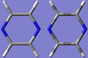
Figure 49. Tube Display Formats
These windows show pyrazine using the the tube display format without (left) and with (right) the Use Bond Color item checked. The format on the left is the default.
The Text Panel
The Text panel of the Display Format dialog controls the font and color of atom labels and symbols as well as allowing you to exclude certain atoms from labeling as previously mentioned. It is illustrated in Figure 50.
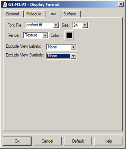
Figure 50. The Text Panel of the Display Format Dialog
This panel allows you to specify various aspects of text labeling of atoms.
The Font File menu allows you to select from several font files provided with GaussView. The Size field specifies the relative type size: type resizes with the molecule as you zoom in or out. The Render field specifies the type rendering method, and the Color field specifies the type color. Note that font sizes are generally limited to those included on the Size menu.
Customizing Display Colors
The Colors preferences allow you to customize the coloring of view window backgrounds, atoms (elements), bonds, surfaces and vibration vector displays. The dialog is illustrated on the left in Figure 51.
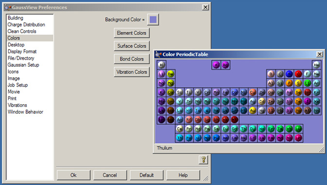
Figure 51. Customizing GaussView Colors
The Colors preferences dialog appears on the left, and the Element Colors preferences appears on the right.
The items in the Colors preferences dialog control the coloring of the following items:
- Background Color: Background color in view windows. Click on the color chip to modify it.
- Element Colors: Element-based atom coloring. This button brings up a periodic table indicating the default color for each element (see Figure 51). Click on any element to change its default color.
- Surface Colors: Specifies colors for surfaces (discussed below).
- Bond Colors: Sets coloring for bonds in each of the various display types. The dialog is similar to the one in Figure 52, and it displays the selected color on a sphere. Don’t be confused by this; the selected colors will be used to color the bonds, not the atoms.
- Vibration Colors: Sets the coloring of the dipole derivative and displacement vectors in vibrations displays. Again, although the color selector is similar to the one in Figure 52, the color selected will be used to color the displayed vectors, not the atoms.
Specifying Colors
The dialog in Figure 52 is used to specify coloring for single-color surfaces. For surfaces types having positive and negative lobes, two colors are specified (as in the figure, which specifies colors for MO surfaces). The dialogs for other Colors preferences items are similar.
The fields at the top of this example dialog allow you to select the surface type and display style (in dialog for other items, the appropriate items are substituted for these). The most important fields are located in the center of the dialog. The Scheme popup allows you to select the type of coloring that is applied to the object. The 1-Color Shaded, 2-Color Shaded, 3-Color Shaded, and 4-Color Shaded items select gradient-filled coloring consisting of shades of the indicated color (1-Color Shaded) or blends between the specified colors (2 or more colors). Keep in mind that less is more with gradients when good taste prevails. The 1-Color Flat colors the object using the specified color in a solid mode, without creating any illusion of three-dimensional shape.
Clicking on any of the color chips in this area allows you to modify that color. Note that two-lobed surfaces will have two sets of color chip(s), placed on the left and right sides of the dialog. If the Use RGB Selector checkbox is selected, then you can use the sliders below it to specify the RGB values for the desired color. If it is unchecked, then the system color picking utility will be invoked.
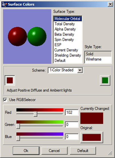
Figure 52. Surface Coloring Preferences
This dialog allows you to customize the colors used for surfaces.
Adding and Synchronizing Views
View=>Add View menu item and the Add View button may be used to add a new view window for the current model. This view is independently adjustable, and begins with the default settings (rather than those of the current view window).
The View=>Synchronize menu item can be used to link distinct views of the same model with respect to mouse-based view operations: rotation, translation, zooming, etc. You must enable this item for each view window that you want to synchronize. Note that synchronization does not affect other display choices and that views are automatically synchronized with respect to structural changes.
Selecting View Windows
The Windows menu contains items which control which view windows are open and/or visible. All views and associated dialogs of a molecule group can be hidden/shown by checking/unchecking the corresponding item in the Windows=>Molecule Groups submenu. Individual view windows can be hidden or shown using the corresponding item at the bottom of the main Windows menu. Selecting a window here makes it the active view. Note that hiding is not the same as closing and is solely for the purpose of managing screen space. It is also different from minimizing a window as no icon is visible for a hidden window.
The Show All and Show None items on the Windows=>Molecule Groups submenu display and hide windows for all model groups (respectively). The related Windows=>Minimize All, Windows=>Restore, and Windows=>Restore All menu items respectively minimize, open the active view, or open all minimized view windows (but not hidden ones). The Windows=>Close and Windows=>Close All items close the active window or all view windows (respectively).
The Windows=>Previous and Windows=>Next items (and the equivalent Previous and Next buttons) activate the previous or next window in sequence.
Finally, the Windows=>Cascade and Windows=>Tile menu items (and the equivalent Cascade and Tile buttons) arrange all windows in an overlapped pile or resize them and rearrange them on the screen so that the maximum number are simultaneously visible (all of them, if possible).
Working with Molecule and Files
In this section, we will discuss operations related to molecules and molecule groups, including their storage in external files.
Pasting Molecules into the View Window
The Edit=>Cut and Edit=>Copy menu items and the corresponding Cut and Copy buttons can be used to cut or copy the entire structure in the current model to the system clipboard. Note that any atom selection within the model is ignored.
The Edit=>Delete Molecule menu item and the Delete Molecule button can be used to remove the structure in the current model, discarding it without copying it anywhere.
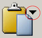
There are several options for pasting molecules from the clipboard. The Edit=>Paste menu item accesses a slideoff menu containing three items. These items can also be reached via the small downward pointing triangle on the Paste button. Clicking on the Paste icon itself (avoiding the triangle’s panel) selects the Replace Molecule item.
The items on the Paste submenu are:
- Edit=>Paste=>Add to Molecule Group: Create a new model within the current molecule group, and place the structure on the clipboard into it.
- Edit=>Paste=>Replace Molecule: Remove the structure in the active window and place the one on the clipboard there instead.
- Edit=>Paste=>Append Molecule: Add the molecule on the clipboard to the active model as a separate fragment.
File Drag and Drop under Windows
On the Windows platform, files can be added to the current molecule group by dragging them from an Explorer window or other source and dropping them onto a view window. Dragging and dropping with the left mouse button will load the contents of each file and add it to the molecule group.
By default, file contents are placed as new molecules within the current molecule group. However, dragging and dropping multiple files with the right mouse button will open a context menu with these options:
- Add all files to this molecule group: The files are appended to the current molecule group (the default).
- Append files to this molecule: The contents of the file(s) are appended to the current molecule (rather than creating new frames within the current molecule group).
- Separate new molecule group for each file: A new molecule groups are created for each file and the current molecule group is unchanged.
- Single new molecule group for all files: One new molecule group is created for all of the files, with each file comprising one molecule (frame) within it, and the current molecule group is unchanged.
The wording of the options differs slightly when only a single file is dragged, and the final option does not appear.
Adding a Model
The File=>New menu item accesses a slideoff menu containing two items. The items on the New submenu are:
- Create Molecule Group: Create a new view window corresponding to the model in a new molecule group.
- Add to Molecule Group: Create a new view window corresponding to an additional model in the current model group.
In both cases, the new view window is initially empty.
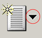
These items can also be reached via the small downward pointing triangle on the New button. Clicking on the New icon itself (avoiding the triangle’s panel) selects the Create Molecule Group item.
Opening Existing Models and Other Files
The File=>Open menu item and the Open button both bring up the Open File dialog. The format of this dialog follows the native form for the local computer, with the addition of some GaussView-specific fields which are illustrated in Figure 53.
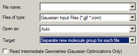
Figure 53. GaussView Fields in the Open File Dialog
GaussView adds three fields and a checkbox to the standard Open File dialog provided by the operating system.
These additional items have the following meanings. The Files of Type popup is used to select the file type to open. It also acts as a filter selecting which files are displayed in the dialog’s file list. The file list will be limited to the files with the selected extension(s). Supported file types include:
- Gaussian Input Files (.com or .gjf)
- Gaussian Output Files (.log or .out)
- Cube Files (.cub)
- Gaussian Checkpoint Files (.chk)
- Gaussian Formatted Checkpoint Files (.fch*)
- Brookhaven PDB Files (.pdb or .ent)
- MDL Mol Files (.mol)
- Sybyl Mol2 Files (.mol2 or .ml2)
- CIF Files (.cif)
All files may also be displayed if desired by selecting the All Files item.
The Open as popup is used to force an input file to be interpreted as the specified file type, regardless of the actual file extension. All supported file types except Gaussian cube files are available as choices here. The default is Auto, which identifies the file type by its extension alone.
The Target popup specifies where the read-in structure should be placed:
- Separate new molecule group for each file: Create a new, one member molecule group for each file that is read in. This is the default.
- Single new molecule group for all files: Create one new molecule group, and make each file a molecule within it. When opening a single file, this is equivalent to the first option.
- Append all files to active molecule: Place the structures from all opened files into the current molecule (in the current molecule group). This will result in additional fragments being added.
- Add all files to active molecule group: Add each file as a separate, new molecule within the current molecule group. The current molecule is left unchanged.
In general, only the first structure present in a file is input. Thus, only the structure in the first job step of Gaussian input files is retrieved. However, when selected, the Read intermediate geometries (optimization only) checkbox causes GaussView to retrieve all geometries that are present in some Gaussian results files as separate models within the designated target. This box applies to results files from geometry optimizations, IRC jobs, ADMP and BOMD trajectory calculations and potential energy surface scans: all jobs with an optimization component. It is not valid with the Append all files to active molecule choice.
Accessing Recent and Related Files
The File=>Recent Files menu path contains a list of files that have been opened most recently. You can specify the number of items in the list with the Maximum Recent Files field in the File/Directory preferences. However, using these shortcuts always reads in only a single geometry from the specified file into a new model group, regardless of the current setting of the current settings in the Open File dialog or the method that was used to open the file on the previous occasion. The file list is saved across GaussView sessions.
The File=>Related Files menu path contains a list of openable files which are related to the active molecule (e.g., Gaussian output file, checkpoint file, and so on).
The File=>Refresh menu path reloads from the current molecule from its original file, centering and possibly reorienting the molecule. It is available only when the current molecule has not been modified.
Viewing the Input File for the Current Results
Pressing the View File button or selecting the Results=>View File menu item opens the file which was opened for the current model, provided that the molecule has not been structurally modified in any way since it was opened. In the case of binary input files like Gaussian checkpoint files, the displayed file will be the one that was created automatically by GaussView with the formchk utility.
Saving Molecules
The File=>Save menu item and the Save button allow you to save the current model to an external file or set of files. These items use the system’s Save dialog, to which GaussView adds some additional fields (see Figure 54).
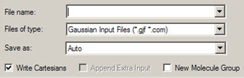
Figure 54. GaussView Fields in the Save File Dialog
GaussView adds several fields to the standard system Save dialog. Molecules can be written in several formats.
These fields have the following meanings:
- Files of type: Acts as a filter, selecting which files are displayed in the dialog’s file list.
- Save as: Forces the saved file to be written as the selected type, regardless of the file extension that it is assigned. The default is Auto, which selects the output file format based on its extension.
- Write Cartesian Coordinates: If checked, the molecular structure is written in Cartesian coordinates in the saved file. By default, a Z-matrix is written.
- Append Extra Input Data: This control is active for models which were read in from Gaussian input files. If there was additional input present in the file, checking this box will cause it also to be included in the output file.
- Create New Molecule Group: If checked, GaussView also creates a new molecule group containing the saved molecule.
Within a molecule group, the current model is saved. There is no way to save all of the molecules within a molecule group to a single file or to a group of files in a single operation.
Printing and Saving Images
Various options on the File and Edit menus, along with the corresponding buttons, can be used to print the contents of view windows and to save their graphical displays as image files.
Printing
The image in the active view window can be printed by selecting File=>Print or clicking on the Print button. The normal operating system Print dialog is then displayed.
Print output is also controlled by settings in the Print preferences, as shown in Figure 55. Settings in the print dialog have precedence over those in the preferences.
The default print operation increases the image resolution to match the printer resolution, up to a maximum factor of 4, and prints the image on a white background. Note that the image always prints at its current size (despite the wording of the second control). If you need to enlarge an image, use the Enlarge Width and Height instead (or in addition). A color image is produced unless Gray Scale is selected.
The Object Quality slider specifies the image quality. Moving the slider toward the Realistic end of the scale increases the file size and the time required to generate the image file. The maximum setting is recommended for publication quality images.
The remaining controls specify low-level graphics behavior. Generic Pixel Format says to use the system software renderer. This option should be checked only after rendering problems/failures have been encountered during image capture or printing. Use Pixel Buffers says to use OpenGL pixel buffers (may improve graphics performance in some implementations).
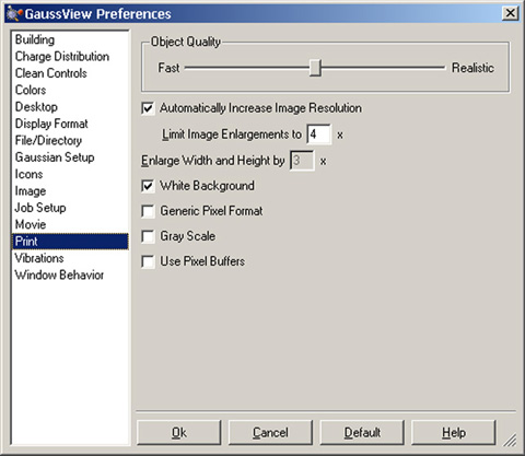
Figure 55. GaussView Print Preferences
This panel allows you to specify that printed images are always enlarged to match the printer resolution (subject to the maximum value in the Limit Enlargements to field) and/or that images always appear on a white background (vs. the background used in its view window), as well as other choices.
Capturing Images and Saving Image Files
The Edit=>Image Capture menu path may be used to capture the image in the current view windows to the system clipboard (from which it may be pasted into another application). The File=>Save Image File menu item and the Save Image button allow you to save an image to an external file. They use the system Save dialog, with some additional fields as shown in Figure 56.
The Files of type field acts as usual as a filter determining what files are displayed in the file list. The Save as field specifies the kind of graphics file to be produced (by default, this is determined from file extension). The available files types are TIFF, JPEG, JPEG2, vector-based EPS, Windows Bitmap and PNG. In general, we recommend selecting TIFF for later high resolution printing and selecting JPEG or PNG for use on the web or in presentations.
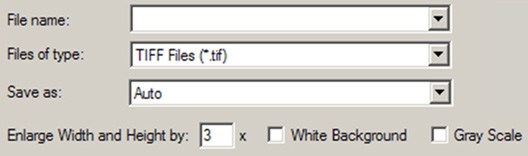
Figure 56. GaussView Fields in the Save Image Dialog
These fields are added to the standard system Save dialog by GaussView when saving images.
The other GaussView fields in the dialog have the following meanings:
- Enlarge Width and Height by: Enlarge the image by uniform scaling in order to increase its physical size and/or graphical resolution (the default value is 3x). Use a factor of 4 if you plan to ultimately print the image at 300 dpi (at its current size). If you also want to increase the image size, you must also include this factor. Thus, to save the current image at 300 dpi at twice its current size, you would use an enlargement factor of 8. Note that the computation time for rendering increases as the square of the enlargement factor.
- White Background: Use a white background. The background in its view window is used if this item in unchecked.
- Use Gray Scale: Convert the image to gray scale (black and white) before saving. The default is to save a color image.
Both the image capture and image saving are subject to the settings in the Image preferences, shown in Figure 57. Settings in the Save dialog override those in the preferences.
The fields in this panel have the following meanings:
- Object Quality: Specifies the image quality. Moving the slider toward the Realistic end of the scale increases the file size and the time required to generate the image file.
- Enlarge Width and Height by: Set the default image scaling factor (as above).
- White Background: Use a white background (the default). The background in its view window is used if this item in unchecked.
- Generic Pixel Format: Use the system software renderer. This option should be checked only after rendering problems/failures have been encountered during image capture or printing.
- Use Gray Scale: Convert the image to gray scale (i.e., black and white) before capturing. The default is to save a color image.
- Use Pixel Buffers: Use OpenGL pixel buffers (may improve graphics performance in some implementations).
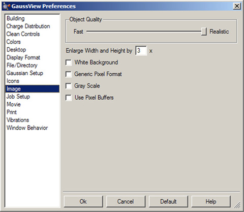
Figure 57. Image Capture Preferences
This panel allows you to set defaults for image captures. Preferences for Movies are similar.
Saving Movies
The File=>Save Movie menu path and the Save Movie button save the various frames in the current molecule group as an animation. The menu path leads to a submenu, which can also be reached by clicking on the small triangle in the button. The submenu has the following selections:
- Save Movie File: Save the frames as a single animation. The available formats are animated GIF and MNG.
- Save Movie Frame Files: Save each frame/molecule within the molecule group as a separate image file. This option is really a shortcut for saving each molecule as an individual image. It is also useful if you want to create your own animation from individual frame files in external software.
- Save Both: Both an animation and the individual frames are saved. You will see two save dialogs in order to specify both files types.
- Clicking on the Save Movie icon on the button selects the Save Movie File choice.
The Movie preferences are similar to those for Images (see Figure 57 above).
Specifying Default File Locations
The File/Directory preferences are illustrated in Figure 58. They allow you to specify the default locations for various kinds of GaussView-related files.
The Starting Directory popup allows you to select the following choices:
- Use previous work directory: Keep track of the last directory visited and use that directory the next time.
- Use launch directory: Always use the directory from which GaussView launched as the default directory.
- Specify: Always use the specified directory.
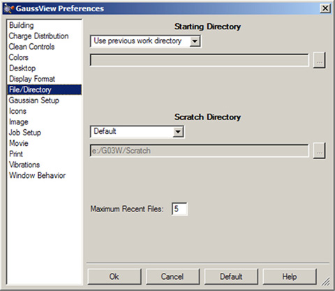
Figure 58. Specifying Default Directory Locations
This dialog allows you to specify default directory locations for file opens and saves, GaussView’s scratch directory and the custom fragment library. It also specifies how many files to include in the recent file list and whether to use filename completion within dialogs (if the operating system supports it).
The Scratch Directory popup, which specifies the location for temporary scratch files that GaussView uses in some cases, has the following choices:
- Use GAUSS_SCRDIR: Use the Gaussian scratch directory for GaussView as well (as defined by the environment variable of this name).
- Use launch directory: Always use the directory from which GaussView launched as the scratch directory.
- Specify: Always use the specified directory as the scratch directory.
Specifying File Associations Under Windows
On Windows systems, the Desktop section of the Preferences dialog allows you to set file associations: file extensions which will be associated with GaussView and for which the application will be opened automatically when such a file is opened. It is illustrated in Figure 59. Note that the file extensions are divided among two panels.
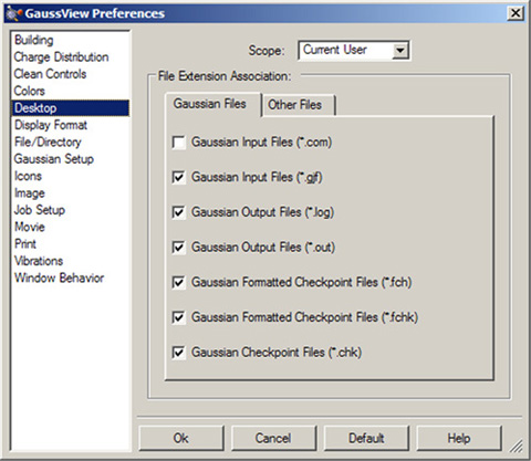
Figure 59. Specifying Windows File Associations
To create a file association between GaussView and the listed Gaussian file type, place a check mark in the associated box. Removing the check mark similarly removes the file association. The Scope fields specifies whether the file association is to affect only the current user or all users on the system.