Matrices or 3D Waves

For more details see Multidimensional Waves, Igor 5 Manual, volume II, p. 123.

Matrices are two-dimensional waves, like a rectangular spreadsheet.
As regular waves, matrices have names and all their entries can be manipulated as a group. While matrices are waves, not all functions and operations useable with 2D waves can be aplied to 3D waves add vise versa.

As with other waves, with matices you can:
• Load or import data
• View and edit data
• Display data
• Address and assign data
• use some practical examples

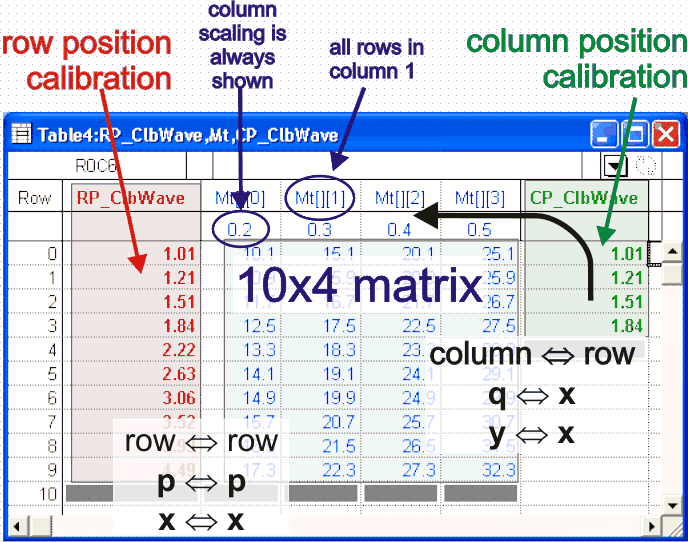
This is a pictorial representaion of a matirx with associated calibration waves:

Importing matrices

Wave import in general is described here for various source programs. Importing matrices is different from importing regular waves in that you can import only one matrix at a time and that structure of data being imported is somewhat predetermined. Data being imported as matrixt contain three parts:

• chunck of data from which matrix is created
• calibration values for rows (may not be present)
• calibration values for columns (may not be present)

Calibration waves are always named from matrix base name by adding CP_ and RP_ prefixes for row and column positions. It is always best to choose a descriptive name for a wave, but even more so for matrix because you may need to rename three seprate waves if you change your mind down the road.

When waves are imported, Igor prints a report in the history window (Ctrl+J). Verify that number of columns and rows actually loaded matches what you are expecting to see.

Editing matrices

Matrices can be diplayed in a table and their values can be edited. This is true for both data that you import from other programs and matrices that you generate manually by typing in values.

When matrices are dipalyed in a table, entire matrix is displayed. Each data column is displayed as a separate column on a table. This means that if yout matrix has 500 spectra, expect that many columns in a table.

When displaying a matrix in a table you can choose if you want to show scaled row calibration (x). Scaled column calibration (y), though, is always shown. In most of our applicaitons scaling is not the best way to calibrate data and left alone column scaling it will default to column number. In either case column title will indciate order position in brackets as is shown in the above illustration.

Displaying matrices

Displaying matrices has more differences form other aspects of their handling than other operations. For once, there are more ways to display a matrix than a regular wave. Because matrix of data can represent a surface or an image, you can display a matrix in 3D views and their projections. In current version of Igor you are limited, though, in your choice of using calibration waves in 3D views. 3D views are useful for getting overall, intuitive impression of the data, but typically too busy for practical presentation in print.

In 2D graphs you can plot any row or column of a matrix by, but only if you use advanced plotting. To plot a slice of a matrix it has to be reduced a regular wave by specifying a single column as in MyMatrix[][5] or a single row as in MyMatrix[5][]. Such slices can be plotted by themselves (against calculated calibration) or against proper calibration wave as X-Y pair. You can append various slices of a matrix to the same plot as many times as you need. For a large number of slices it is practical to use macros.

Accessing data in matrices

Data in matrices are accessed and addressed just as in "regular" waves, except that you typically need to specify position in additional dimension—columns—in the second set of address brackets.  The biggest practical difficulty is memorizing the order in which dimensions are specified.

The mnemonics that can help with this is that as we write, brackets are added as dimensions are added. First set of brackets is present in all waves; second dimension adds the second set of brackets; thirds dimension adds third set etc. Each new dimension also adds one each of position and scaling variables, as described for regular waves here, incrementing them alphabetically. Here is practical summary for the first three dimensions:

Practical use

Have a frequent-use example? Send a suggestion!